D-Optimality with Level Balance Constraints

Andrew Armstrong, Alex Graber

Background: What is Choice Research?

Let’s say you’re having trouble deciding what to have for dinner. You know you want a pasta dish, but you don’t know which dish - there are so many options! You have to choose the noodle shape, the sauce, and what kind of topping you want.

Pasta
Pasta Options (source: google image search)

Choice research could help you make your decision. Using the conjoint method of choice research, you could ennumerate the various options for each attribute and come up with a map defining a pasta dish based on the various attributes:

Pasta Design
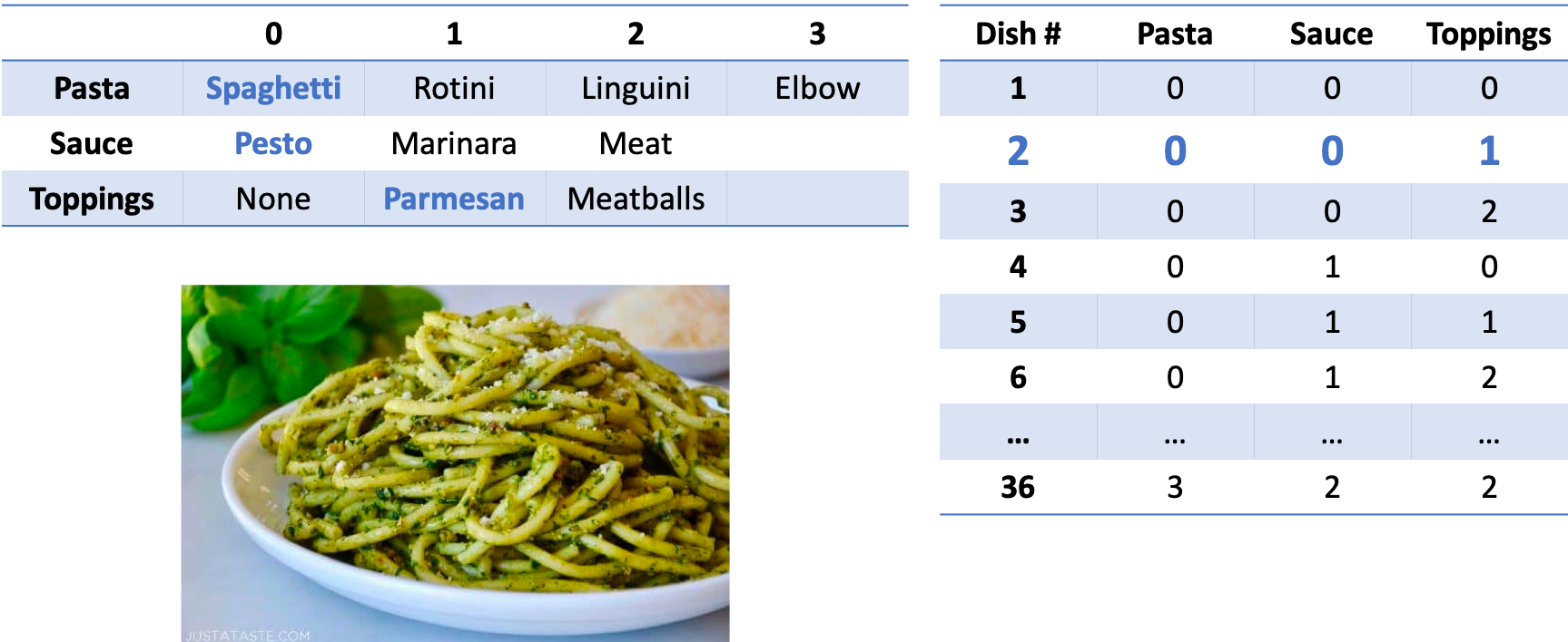
Pasta Choice Design

Notice how the pasta dish in the picture is dish #2 in the chart on the right; it is composed of Spaghetti (pasta level 0), Pesto (sauce level 0), and topped with Parmasen Cheese (topping option 1).

If you had to try every possible pasta dish in the world, it would be impossible - there are so many types! But by defining pasta by its attributes, you can select a small subset of the entire variety and use a multinomial logit model to understand which attributes are your favorite. Then, you could make yourself your personal ultimate pasta dish by combining all of your favorite attributes.

D-Optimality

The pasta story is a simplistic example of choice research, but it should give you the intuition for why choice research is important, and how you can use a smaller portion of all possible options to associate value or importance with attribute levels. This raises a key question: How can you identify the best subset to use that maximizes the information gained from the research?

It is clear that when the number of attributes and levels grow beyond a small set, presenting the full design (full factorial) becomes a challenge due to both the number of combinations required and the amount of burden placed on the respondent. Fractional factorial designs, then, seek to allow the research to eke as much data out of the analysis as possible but use a much more limited subset of stimuli – but how do we know what the best (i.e., most efficient) fractional factorial design is?

Much research has been done on the topic of identifying efficient experimental designs (Hauser & Rao, 2002). The current standard used to identify ‘efficient design’ is D-error – the geometric mean of the eigenvalues of the covariance matrix (D-efficiency is the inverse of D-error) (Kuhfeld, Huber, & Zwerina, 1996). Thus, the goal of an efficient design is to minimize D-error (therefore maximizing D-efficiency).

D-efficient designs satisfy four principles (Kuhfeld, Huber, & Zwerina, 1996):

Orthogonality is satisfied when the levels of each attribute vary independently of one another.
Level balance is satisfied when the levels of each attribute appear with equal frequency.
Minimal overlap is satisfied when the alternatives within each choice set have nonoverlapping attribute levels.
Utility balance is satisfied when the utilities of alternatives within choice sets are the same.

The standard method to identify an efficient design is to use one of any variant of the Fedorov Algorithm which, given a starting design, recursively makes exchange(s) that reduce D-error until some convergence criteria is met. This method is susceptible to local minima; it may be necessary to run multiple iterations of the Fedorov Algorithm with different random starting designs to find the most efficient design (Kuhfeld, Huber, & Zwerina, 1996).

Business Problem

A pharmaceutical market research firm uses simulated patient treatment as a method to understand physician demand in specific treatment areas. In this method, a limited universe of patients is designed in order to represent as much of the actual disease area patient universe as possible. Patients are defined by multiple attributes (age, gender, BMI, etc.), and each attribute may have multiple levels (male/female, etc.). The distribution of attribute levels is controlled such that the demographics of the simulated patient universe approximate the real patient universe. These simulated patients are then treated, where a given treatment (yes/no) can be related back to the patient design.

Patient simulation research in this manner is a specialized choice methodology somewhat analogous to conjoint. In both conjoint and patient simulation, respondents are forced to make a decision based on a stimulus that is composed of multiple attributes and levels (Kuhfeld, Huber, & Zwerina, 1996). There are two key differences between conjoint (the pasta example) and patient simulation:

The design for patient simulation inherently contains d-error as a result of violating the principle of level balance: Since the goal is for the simulated patient universe to map to the actual patient universe, the researcher may need to control for the distribution of levels within each attribute.
Certain attributes and levels may have required interactions (i.e., a patient must be female to be pregnant), potentially violating orthogonality and minimal overlap.

Adding Constraints, Pt 1

Toy Problem

As a toy problem, let us consider a patient universe in which patients are defined by:

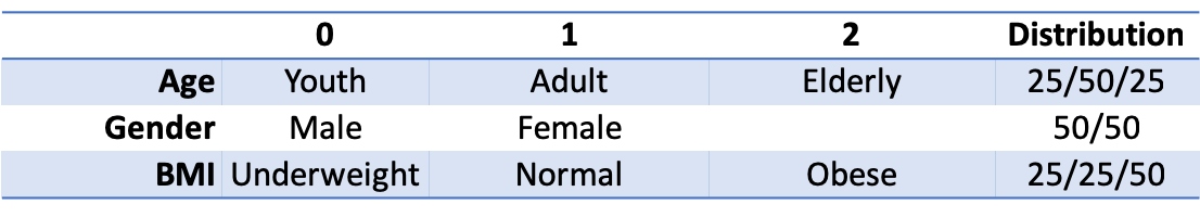
Expanding out all possibilities into the entire candidate set, this would be 3*3*2*3 = 54 unique patient profiles. Given respondent time is expensive, and high respondent burden decreases quality of results, we seek to reduce time-in-survey by creating a fractional-factorial design of 8 unique patient profiles. As we want to extract as much data from the exercise as possible, the 8-profile fractional-factorial design must be as efficient as possible.

Practically speaking, the number of attributes is limited to no more than 25, each with at most 5 levels due to the complexity of the simulation, limited respondent pool, and limited number of experiments possible per respondent. Thus, at most, the candidate set contains $5 ^ { 25 }$ (approx. $3 \times 10 ^ { 17 }$ ) possibilities – and will generally be significantly smaller as not all 25 attributes are used and most contain fewer than 5 levels. However, the worst-case scenario requires approximately $2 \times 10 ^ { 10 }$ gigabytes to merely store the candidate set. The combinatorics problem explains why stochastic search algorithms such as simulated annealing or genetic algorithms are frequently used instead of an exhaustive search against a complete candidate set.

Model Definition

Our goal is to maximize the weighted d-optimality of the design matrix, penalized for missing distributions and impossible variable interactions, and subject to the distributions of each attribute’s levels and interactions, where each attribute’s level is represented by a binary variable.

Objective Function (Wanida Limmun, 2012):

$\text { maximize } f ( X ) = 100 \frac { \operatorname { Det } \left( X ^ { T } X \right) ^ { 1 / p } } { N } - \lambda \sum \left| \delta _ { \text { distribution } } \right| - \lambda ^ { 2 } \sum \left| \delta _ { \text {interaction} } \right|$

where $N$ is the number of observations, $\delta$ are vectors of relaxation variables, and $X$ is the design matrix:

$\left[ \begin{array} { c c c } { A _ { 1 } } & { G _ { 1 } } & { B _ { 1 } } \\ { \vdots } & { \vdots } & { \vdots } \\ { A _ { N } } & { G _ { N } } & { B _ { N } } \end{array} \right]$

With decision variables $A, B, G$ representing attributes:

$\qquad$ Age: $A _ { i } , \quad A \in \{ 0,1,2 \} , i = 1 , \ldots , n$ (i.e., the age group classification for each patient i)

$\qquad$ Gender: $G _ { i } , \quad G \in \{ 0,1 \} , i = 1 , \ldots , n$ (i.e., the gender classification for each patient i)

$\qquad$ BMI: $B _ { i } , \quad B \in \{ 0,1,2 \} , i = 1 , \ldots , n$ (i.e., the BMI classification for each patient i)

For easier constraint formulation, we can use the Dantzig-Wolfe reformulation to rewrite our integer variables where the capital letter represents the binary variable series replacing an integer variable, and the lowercase letter represents the integer set of levels permissible for the given attribute:

$\begin{array} { l l } { A _ { i } = \sum _ { 0 } ^ { z } z Z _ { z } , } & { \text { and } \sum _ { 0 _ { y } } ^ { z } Z _ { z } = 1 , \quad Z _ { z } \in \{ 0,1 \} , z \in \{ 0,1,2 \} } \\ { G _ { i } = \sum _ { 0 } ^ { y } y Y _ { y } , } & { \text { and } \sum _ { w ^ { 0 } } ^ { z } Y _ { y } = 1 , \quad Y _ { y } \in \{ 0,1 \} , y \in \{ 0,1 \} } \\ { B _ { i } = \sum _ { 0 } ^ { w } w W _ { w } , } & { \text { and } \sum _ { 0 } ^ { w ^ { 0 } } W _ { w } = 1 , \quad W _ { w } \in \{ 0,1 \} , w \in \{ 0,1,2 \} } \end{array}$

Subject to:

$\qquad$ Age group proportions:

$\begin{array} { l } { \frac { \sum Z _ { 0 } } { N } = .25 + \delta _ { Z 0 } } \\ { \frac { \sum Z _ { 1 } } { N } = .5 + \delta _ { Z 1 } } \\ { \frac { \sum Z _ { 2 } } { N } = .25 + \delta _ { Z 1 } } \end{array}$

$\qquad$ Gender proportions:

$\begin{array} { l } { \frac { \sum Y _ { 0 } } { N } = .5 + \delta _ { Y 0 } } \\ { \frac { \sum Y _ { 1 } } { N } = .5 + \delta _ { Y 0 } } \end{array}$

$\qquad$ BMI proportions:

$\begin{array} { l } { \frac { \sum W _ { 0 } } { N } = .25 + \delta _ { W 0 } } \\ { \frac { \sum W _ { 1 } } { N } = .25 + \delta _ { W 1 } } \\ { \frac { \sum W _ { 2 } } { N } = .5 + \delta _ { W 2 } } \end{array}$

$\qquad$ Binary constraints: $W , Y , Z \in \{ 0,1 \}$

$\qquad$ Interaction slacks: While not specified in the toy problem, it is entirely possible that we may have interactions specified in the design (i.e., men cannot be pregnant). In these cases, the slacks are the count of the impossible interactions. We will penalize these interaction slacks twice because they are more costly to the design than a missed distribution.

Constrained D-Optimality

For our discrete-choice design, the information matrix of an n-point design is

$\mathrm { M } = X _ { n } ^ { T } X _ { n }$

where $X$ is an $n \times p$ design matrix. Use

$d \left( x _ { i } \right) = x _ { i } ^ { T } \left( \mathrm { X } _ { n } ^ { T } \mathrm { X } _ { n } \right) ^ { - 1 } x _ { i }$

as variance estimator, where $\mathcal { X } _ { i }$ represents a row. See (Labadi, 2015; Triefenback, 2008) for more details regarding optimality theory.

To perform a sequential switch, a ‘delta function’ is defined that allows a less expensive update to the objective function value through the determinant of the information matrix as well as a variance estimator for the swap (Triefenback, 2008):

$\begin{array} { l } { \Delta \left( x _ { i } , x _ { j } \right) = d \left( x _ { j } \right) - \left[ d \left( x _ { i } \right) d \left( x _ { j } \right) - d \left( x _ { i } , x _ { j } \right) ^ { 2 } \right] - d \left( x _ { i } \right) } \\ { \operatorname { det } \left( X _ { n e w } ^ { T } X _ { n e w } \right) = \operatorname { det } \left( X _ { o l d } ^ { T } X _ { o l d } \right) * \left( 1 + \Delta \left( x _ { i } , x _ { j } \right) \right) } \end{array} \\ d \left( x _ { i } , x _ { j } \right) = x _ { i } ^ { T } \left( \mathrm { X } _ { n } ^ { T } \mathrm { X } _ { n } \right) ^ { - 1 } x _ { j } = x _ { j } ^ { T } \left( \mathrm { X } _ { n } ^ { T } \mathrm { X } _ { n } \right) ^ { - 1 } x _ { i }$

In order to update our objective function at each iteration, we use the value $1 + \Delta$ as the ratio between the new and old objective function value. This allows us to pick out row swaps at each iteration that maximize the increase in the objective function. However, we must alter this ratio if we want to penalize the slacks on our proportions in our objective function, while picking out rows that both maximize the increase in the objective function minimize this penalty:

$\begin{array} { c } { \operatorname { det } \left( X _ { n e w } ^ { T } X _ { n e w } \right) - \lambda \sum \delta _ { n e w } = \operatorname { det } \left( X _ { o l d } ^ { T } X _ { o l d } \right) * \left( 1 + \Delta \left( x _ { i } , x _ { j } \right) \right) - \lambda \sum \delta _ { n e w } } \\ { p _ { n e w } = \lambda \sum \delta _ { n e w } , p _ { o l d } = \lambda \sum \delta _ { o l d } } \end{array} \\ \operatorname { det } \left( X _ { n e w } ^ { T } X _ { n e w } \right) - p _ { n e w } = \operatorname { det } \left( X _ { o l d } ^ { T } X _ { o l d } \right) * \left( 1 + \Delta \left( x _ { i } , x _ { j } \right) \right) - p _ { n e w } \\ \operatorname { det } \left( X _ { o l d } ^ { T } X _ { o l d } \right) - \lambda \sum \delta _ { o l d } = \operatorname { det } \left( X _ { o l d } ^ { T } X _ { o l d } \right) - p _ { o l d } \\ \frac { \operatorname { det } \left( X _ { n e w } ^ { T } X _ { n e w } \right) - p _ { n e w } } { \operatorname { det } \left( X _ { \text {old} } ^ { T } X _ { \text {old} } \right) - p _ { \text {old} } } = \frac { \operatorname { det } \left( X _ { \text {old} } ^ { T } X _ { o l d } \right) * \left( 1 + \Delta \left( x _ { i } , x _ { j } \right) \right) - p _ { \text {new} } } { \operatorname { det } \left( X _ { \text {old} } ^ { T } X _ { \text {old} } \right) - p _ { \text {old} } }$

Therefore, we can define a new update criterion:

$\begin{array} { c } { \Delta _ { p } \left( x _ { i } , x _ { j } \right) = \frac { \operatorname { det } \left( X _ { o l d } ^ { T } X _ { o l d } \right) * \left( 1 + \Delta \left( x _ { i } , x _ { j } \right) \right) - p _ { n e w } } { \operatorname { det } \left( X _ { o l d } ^ { T } X _ { o l d } \right) - p _ { o l d } } - 1 } \\ { \operatorname { det } \left( X _ { n e w } ^ { T } X _ { n e w } \right) - p _ { n e w } = \left( \operatorname { det } \left( X _ { o l d } ^ { T } X _ { o l d } \right) - p _ { o l d } \right) * \left( 1 + \Delta _ { p } \left( x _ { i } , x _ { j } \right) \right) } \end{array}$

This criterion allows us to figure out the row swap that maximizes our objective function, given that the slacks are penalized. It also allows us to terminate the algorithm as the improvement $\Delta _ { p }$ converges to zero, i.e. the marginal improvement of another swap becomes trivial.

Modified Fedorov Algorithm

We have implemented a modified Fedorov Algorithm (Labadi, 2015; Triefenback, 2008) that considers the slack of distribution constraints (step 4) when performing the iterative state search:

Calculate the candidate set, the set of all theoretically possible combinations. Because of the possibility of explosive growth with combinatorics, this will not always be feasible.
Generate an initial n-point design (an arbitrary design with a nonsingular information matrix) that generally obeys distribution constraints
Compute $M, M ^ { \top }$ , and the determinant of $M$
Perform an exhaustive search across the design matrix $X$ and the entire candidate set, using the delta function and $\Delta _ { p } \left( \mathbf { x } _ { i } \mathbf { x } _ { j } \right)$ to identify the pair of points that maximally improve D-optimality, penalizing the slack from the distribution constraints. Perform the swap.
If efficiency metric is sufficiently close to optimal (or improvement from variance estimator is sufficiently small), stop. If the iteration limit is reached, stop. Set $i = i + 1$ and return to step 3

Fedorov Code

### NOTE: custom Fedorov Design Class is used.  See https://github.com/ahgraber/Fedorov for full code package
#-- Objective functions -----------------------------------------------------------
doptimality <- function(dm, design, lambda=0) {
  # calculates doptimality of design (and optionally penalizes distribution constraints)
  # params:
  # dm: DesignMatrix object containing attribute & constraint information
  # design: design matrix where columns are attributes and rows are patients
  # lambda: weight to penalize constraints.  lambda=0 means no distribution constraints
  # returns: d-efficiency metric
  
  # calculate slacks for the design
  dm$X <- design
  dm$update_slacks()

  objective <- (100 * det( t(design)%*%design )^(1/ncol(design)))/ nrow(design)
  # objective <- det( t(design)%*%design ) / nrow(design)
  penalty <- lambda*( sum(abs(unlist(dm$dslacks))) + lambda*(sum(abs(unlist(dm$islacks)))) )
  # this double-penalizes islacks b/c we really don't want impossible interactions
  return(objective - penalty)
}

#-- Helper functions -----------------------------------------------------------
# d <- function(D, row) {
#   # function to calculate variance estimator
#   # params:
#   # D: current design matrix
#   # row: row to evaluate wrt. design
#   estimator <- row %*% solve( t(D)%*%D ) %*% t(row)
#   return(estimator)
# }

var_est <- function(D,i_row,j_row) {
  # variance estimator for swapping rows
  # params:
  # D: current design matrix
  # i_row: leaving row
  # j_row: entering row
  
  # attempting protection from singular matrix inversions
  X <- tryCatch( 
    { solve( t(D)%*%D ) },
    finally={ MASS::ginv( t(D)%*%D )  }
  )    
  est <- j_row %*% X %*% i_row
  return(est)
  # return(j %*% solve( t(as.matrix(D))%*%as.matrix(D) ) %*% t(as.matrix(i)))
}

penalty <- function(dm, X, lambda) {
  # penatly calculator
  # params:
  # dm: DesignMatrix object with attributes and constraints
  # X: design matrix
  # lambda: penalty for slacks
  # returns: penalty
  
  # calculate slacks for the current design
  dm$update_slacks()
  
  penalty <- lambda*( sum(abs(unlist(dm$dslacks))) + lambda*(sum(abs(unlist(dm$islacks)))) )
  return(penalty)
}

delta_var <- function(D, i, j, lambda) {
  # variance estimator for swapping rows
  # params:
  # D: current design matrix
  # i: leaving row
  # j: entering row
  # lambda: penalty for slacks
  # returns: variance estimator
  
  est <- var_est(D,j,j) - ( var_est(D,j,j)*var_est(D,i,i)-var_est(D,i,j)^2 ) - var_est(D,i,i)
  return(est)
}

update_obj <- function(D, i, j_row, lambda, det, dvar) {
  # calculates the % increase in the objective function for the row swap
  # params:
  # D: current design matrix
  # i: leaving row *index*
  # j: entering row
  # lambda: penalty for slacks
  # det: determinant
  # dvar: delta variance estimator
  # returns: updated doptimality metric
  
  # calculate penalties
  old_p <- penalty(dm, D, lambda)
  i_row <- D[i,]
  dm$del_row(i)
  dm$add_row(j_row)
  dm$update_slacks()
  new_p <- penalty(dm, dm$X, lambda)
  
  # revert dm$X
  dm$X <- D 
  return( (det*(1+dvar)-new_p) / (det-old_p) - 1 )
}

#-- Fedorov --------------------------
fedorov <- function(dm, candidate_set, n, lambda=0) {
  # fedorov algorithm find d-optimal design
  # params:
    # dm: Design Matrix object
    # candidate_set: matrix of all possible combinations of attributes
    # n: number of rows
    # lambda: weight for slack penalties
  # returns: optimal design
  
  # set inital values of algorithm
  iter <- 1
  obj_delta_best <- .0001
  det <- as.numeric(determinant(t(dm$X)%*%dm$X)$modulus)
  
  # iterate until the improvement in D-optimality is minimal or 100 iterations is reached
  while ((obj_delta_best > 10e-6) && (iter < 100)) {

    i_best <- NULL
    j_best <- NULL
    obj_delta_best <- 0
    
    for (i in 1:n) {                      # iterate through rows in design matrix
      for (j in 1:nrow(candidate_set)) {  # iterate through rows in candidate set
        
        dvar <- NULL
        obj_delta <- NULL    

        # calculate the potential improvement in D-optimality by replacing the
        # current row in the design with the current row in the candidate set
        dvar <- delta_var(dm$X, dm$X[i,], candidate_set[j,])
        # delta <- delta_var(dm$X, t(dm$X[i,]), as.matrix(candidate_set[j,]))
        obj_delta <- update_obj(dm$X, i, candidate_set[j,], lambda, det, dvar)

        # if that is greater than the best candidate so far, make it the new best pair
        if (obj_delta > obj_delta_best) {
          obj_delta_best <- obj_delta
          dvar_best <- dvar
          i_best <- i
          j_best <- j
          print(paste(paste("iteration", iter, sep=" "), obj_delta_best, dvar_best, sep=" | "))
        } else {
          next
        }
      } # end for j
    } # end for i

    ### updates
    if (is.null(i_best)) {
      # no better swaps found
      break
    } else {
      # perform swap
      dm$del_row(i_best)
      dm$add_row(candidate_set[j_best,])
      dm$update_slacks()
      
      # update the determinate following the swap
      det <- det*(1+dvar_best)
      
      iter <- iter+1
    }
    
  } # end while
  
  if (iter == 100) {
    print("Algorithm stopped due to reaching iteration limit")
  } else {
    print(paste("Convergence achieved in ",iter," iterations"))
  }
  return(dm$X)
} # end fedorov

Parallelized

We attempted to then parallelize the modified Fedorov Algorithm as it has ‘embarrassingly parallel’ tasks in the exhaustive search. In step 4 above, it should be possible to calculate $\Delta _ { p } \left( \mathbf { x } _ { i } \mathbf { x } _ { j } \right)$ in parallel. Our R implementation fails, seemingly due to a bug in the doParallel or foreach libraries that prevent passing a reference class object to the parallel environment. While the parallel infrastructure may require too much overhead to outperform the non-parallel version for the toy problem (especially given that we must store $\Delta _ { p } \left( \mathbf { x } _ { i } \mathbf { x } _ { j } \right)$ for each pair and sort the final list), we believe that as the problem size grows, the effects of parallelizing would show significant runtime improvements.

MFA Results

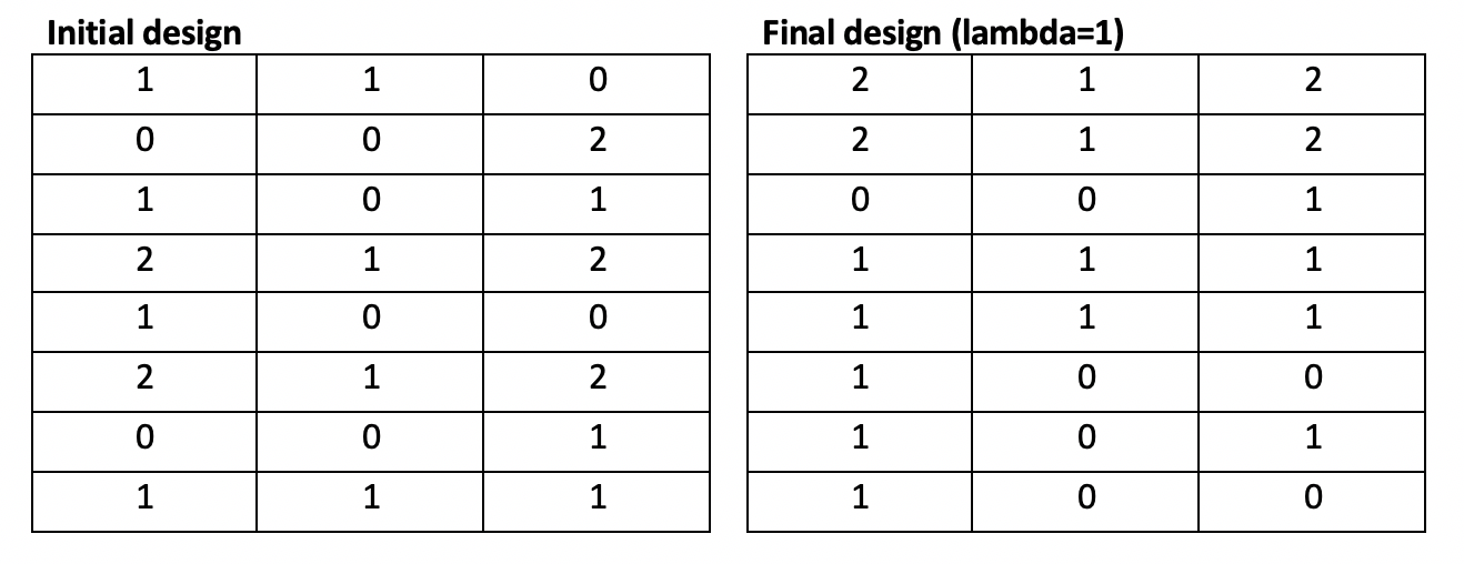
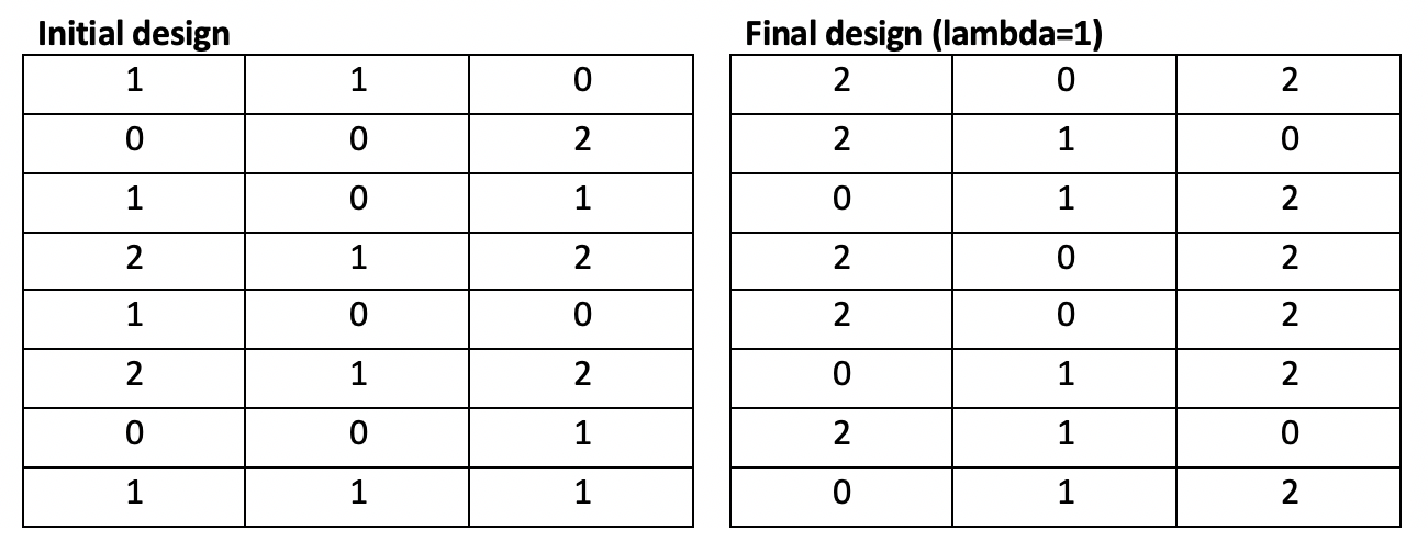
Running the modified Fedorov Algorithm for our toy problem on a top-of-the-line computer requires approximately 25 seconds per 100 iterations. With lambda > 0, It becomes evident that oscillation is present, and the toy problem stops due to reaching the iteration limit, not due to convergence. Additionally, the d-optimality of the resulting design (35.3) actually makes the design worse compared to the initial, randomly-generated design (53.1).

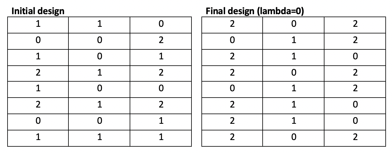
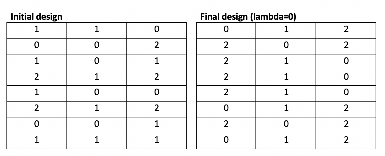
With lambda = 0 (no penalty; normal Fedorov Algorithm), the algorithm converges in 10 iterations over 2 seconds and demonstrates a significant improvement in d-optimality (131.0) over the original random design (53.9).

Both storage and runtime requirements limit the utility of this algorithm. For large problems, it is infeasible to store the entirety of the candidate set; even if storage were possible, exhaustively iterating across $3 \times 10 ^ { 17 }$ possibilities (as defined in our worst-case scenario) would require more time than any user is likely to be willing to spend.

Genetic Algorithm

Given the infeasibilities associated with running a discrete, exhaustive search on large candidate sets, we have also implemented a genetic algorithm to perform a stochastic search (Wanida Limmun, 2012):

Generate the initial herd of size population – a list of randomly generated designs
Calculate the d-optimality of each. Preserve some number of elites.
Breed random pairs of the non-elite stock (i.e., generate 2 new designs with random 50% from each parent).
Randomly mutate cells within the children.
Recombine the herd and assess the fitness (d-optimality) of each. Cull the poor performers, keeping only population.
Identify the most fit of the new generation; compare fitness to best from prior generation. If fitness increase is sufficiently large, increment the number of generations and go back to step 2. Otherwise stop. If the maximum number of generations is reached, stop.

Steps 2, 3, 4, and 5 are all ‘embarrassingly parallel’, so it is possible to implement a parallelized genetic algorithm to allow faster traversal of the search space or larger populations and more generations.

Fedorov Code

### NOTE: custom Fedorov Design Class is used.  See https://github.com/ahgraber/Fedorov for full code package
#-- Objective functions -----------------------------------------------------------
doptimality <- function(dm, design, lambda=0) {
  # calculates doptimality of design (and optionally penalizes distribution constraints)
  # params:
  # dm: DesignMatrix object containing attribute & constraint information
  # design: design matrix where columns are attributes and rows are patients
  # lambda: weight to penalize constraints.  lambda=0 means no distribution constraints
  # returns: d-efficiency metric
  
  # calculate slacks for the design
  dm$X <- design
  dm$update_slacks()
  
  objective <- (100 * det( t(design)%*%design )^(1/ncol(design)))/ nrow(design)
  # objective <- det( t(design)%*%design ) / nrow(design)
  penalty <- lambda*( sum(abs(unlist(dm$dslacks))) + lambda*(sum(abs(unlist(dm$islacks)))) )
  # this double-penalizes islacks b/c we really don't want impossible interactions
  return(objective - penalty)
}

#-- supporting functions ---------------------------------------
breed <- function(X, Y){
  # breeding function for genetic algorithm; approx 50/50 mix of parents
  # params:
    # X: design matrix (parent 1)
    # Y: design matrix (parent 2)
  # returns:
    # list(A,B) where A,B are child matrices of X,Y
  
  if (nrow(X) != nrow(Y)) {stop('Parents do not have equivalent rows')}
  if (ncol(X) != ncol(Y)) {stop('Parents do not have equivalent columns')}
  
  probsA <- runif(nrow(X),0,1)
  ax <- X[probsA > .5,]  # chromosomes from parent X
  ay <- Y[probsA <= .5,] # chromosomes from parent Y
  A <- rbind(ax,ay)

  probsB <- runif(nrow(X),0,1)
  bx <- X[probsB > .5,]  # chromosomes from parent X
  by <- Y[probsB <= .5,] # chromosomes from parent Y
  B <- rbind(bx,by)
  
  return(list(A,B))
} # end breed
mutate <- function(dm, X, alpha) {
  # mutation function for genetic algorithm
  # params:
    # dm: Design Matrix object
    # X: design matrix (chromosome to be mutated)
    # alpha: num 0-1 indicating likelihood for mutation (lower increases mutation)
  # returns: mutated matrix X
  
  for (i in 1:nrow(X)){
    # test whether to mutate row
    if (runif(1,0,1) >= alpha) { 
      for (j in 1:ncol(X)) {
        # test whether to mutate cell
        if (runif(1,0,1) >= alpha) {
          # pick new value from permissible levels of attribute column
          X[i,j] <- sample(c(1:dm$levels[j]-1),1)
        } # end if j
      } # end for j
    } # end if i
  } # end for i
  
  return(X)
} # end mutate
cull <- function(elite, stock, children, pop, dir) {
  # function to reduce population back down to pop
  # params:
    # elite: list of elite design matrices to be preserved
    # stock: list of non-elite parents design matrices
    # children: list of new design matrices
    # pop: int, population size to achieve
  # returns: list (length pop) of best design matrices
  
  # combine stock and child lists
  fill <- append(stock,children) 
  fill <- sorter(fill, dir)
  
  # find number of herd to fill after elites are kept
  nfill <- pop-length(elite) 
  
  # generate new herd with elites and best of rest
  herd <- append(elite, head(fill, nfill))

  return(sorter(herd, dir))
} # end cull
sorter <- function(herd, dir) {
  # function to sort the herd based on objective function
  # params:
  # herd: list of (dval, matrix) tuples to be sorted
  # dir: direction to sort
  # returns: sorted herd
  
  if (dir=="min") {
    # value <- sapply(herd, function(x) x[[1]])
    # herd[order(value, decreasing=T)]
    return(herd[order(sapply(herd, function(x) x[[1]]), decreasing=F)])
  } else if (dir=="max") {
    # value <- sapply(herd, function(x) x[[1]])
    # herd[order(value, decreasing=T)]
    return(herd[order(sapply(herd, function(x) x[[1]]), decreasing=T)])
  } else {
    stop("Direction for objective function not defined")
  }
} # end sorter

# genetic algorithm
gen_alg <- function(dm, pop, gens, test, lambda=0) {
  # genetic algorithm to find d-optimal design
  # params:
    # dm: Design Matrix object
    # pop: population size
    # gens: int, maximum number of generations
    # test: objective function to use
  # returns: optimal design
  
  if (pop < 16){ stop('Suggested population minimum of 16') }
  if (gens < 100){ stop('Suggested generation minimum of 100') }
  
  if (test=="doptimality"){
    objfun <- doptimality
    dir <- "max"
  } else if (test=="sumfisherz") {
    objfun <- sumfisherz
    dir <- "min"
  } else {
    stop("Test value not in c('doptimality','sumfisherz')")
  }

  alpha <- 0.4 # probability threshold; lower increases variation/mutation

  ### create herd (list of (dval, matrix) tuples)
  herd <- list()
  for (p in 1:pop) {
    dm$generate()
    herd[[p]] <- list(objfun(dm, dm$X, lambda), dm$X)
  }
  herd <- sorter(herd, dir)
  top <- herd[[1]]
  
  ### pick elite designs to leave unchanged/unculled
  if (pop < 32) { 
    nelite <- 2 
  } else { 
    nelite <- 4
  }
  
  g <- 1  # initialize iterator
  converge <- 0 # initialize convergence criteria counter
  while ((g < gens) && (converge < log2(gens))) {
    # stop if reach maximum generations OR 
    # if difference between top designs remains small for some number of generations
          
    if ((pop %% 2) != 0) { nelite <- nelite-1} # adjust for odd population
    elite <- head(herd, nelite)
    stock <- tail(herd, -nelite)
    
    ### breed randomized pairs
    x <- sample(c(1:length(stock)))
    y <- sample(c(1:length(stock)))
    children <- list()
    for (i in 1:length(stock)) { 
      if (x[i] != y[i]) { # no self-replication
        if (runif(1,0,1) >= alpha){
          # if test passed, breed & save children
          kids <- breed(stock[[ x[i] ]][[2]],stock[[ y[i] ]][[2]]) 
          children[[length(children)+1]] <- kids[[1]]
          children[[length(children)+1]] <- kids[[2]]
        }
      }
    } # end for i (breed)
    
    ### mutation
    for (j in 1:length(children)) { 
      if (runif(1,0,1) >= alpha) {
        # if test passed, mutate child
        children[[j]] <- mutate(dm, children[[j]], alpha)
      }
    } # end for j (mutate)

    ### assess fitness
    for (k in 1:length(children)) {
      children[[k]] <- list(objfun(dm, children[[k]], lambda), children[[k]])
    }
    
    ### cull
    herd <- cull(elite, herd, children, pop, dir)

    ### updates
    g <- g+1
    if (dir == "max") {
      if ((herd[[1]][[1]]-top[[1]]) < 10e-6 ) {
        # maximizing, so change should be positive
        # if the change in objval (new - old) 0 and small pos number, system is converging
          # smallest possible change is 0 (i.e., same best design) b/c preserving elites
        # if converging, count as a converge step to potentially break out of while loop
        converge <- converge+1
      } else {
        # if not a converge step, reset converge coutner to 0
        converge <- 0
      }
    } else if (dir == "min") {
      if ((herd[[1]][[1]]-top[[1]]) > -10e-6 ) {
        # minimizing, so change should be negative
        # if the change in objval (new - old) small neg number and 0, system is converging
          # largest possible change is 0 (i.e., same best design) b/c preserving elites
        # if converging, count as a converge step to potentially break out of while loop
        converge <- converge+1
      } else {
        # if not a converge step, reset converge coutner to 0
        converge <- 0
      }
    }

    top <- herd[[1]]
  } # end while
  
  print(paste("Convergence achieved in ",g," iterations"))
  return(herd[[1]])
} # end gen_alg

GA Results

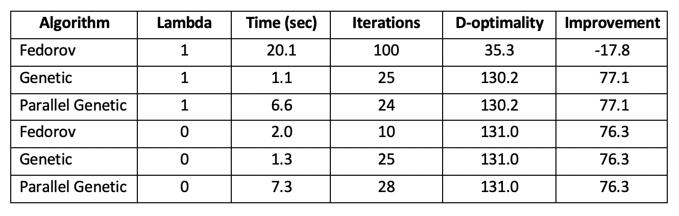
These algorithms outperform our implementations of the modified Fedorov Algorithms. With lambda=1, our genetic algorithm converges in 22 iterations taking 1.1 seconds to a solution with d-optimality 131 (significantly better than the Fedorov Algorithm, and close to the Fedorov Algorithm’s optimal solution with lambda=0).

With lambda=0 (no penalty), the genetic algorithm converged in an equivalent 22 iterations over 1.1 seconds to a solution with d-optimality 131, matching the Fedorov Algorithm’s performance in a fraction of the time.

The parallelized genetic algorithm finds the same solutions but takes approximately 6 times longer due to the overhead of parallelization. With a larger problem, this overhead becomes negligible and parallelization becomes an asset.

Adding Constraints, Pt 2

Full Problem

As mentioned previously, the number of attributes in the full problem is generally limited to no more than 25, each with at most 5 levels due to the complexity of the simulation, limited respondent pool, and limited number of experiments possible per respondent. For a Type 2 Diabetes study, we might define patients with 16 attributes, each containing between 2-4 levels:

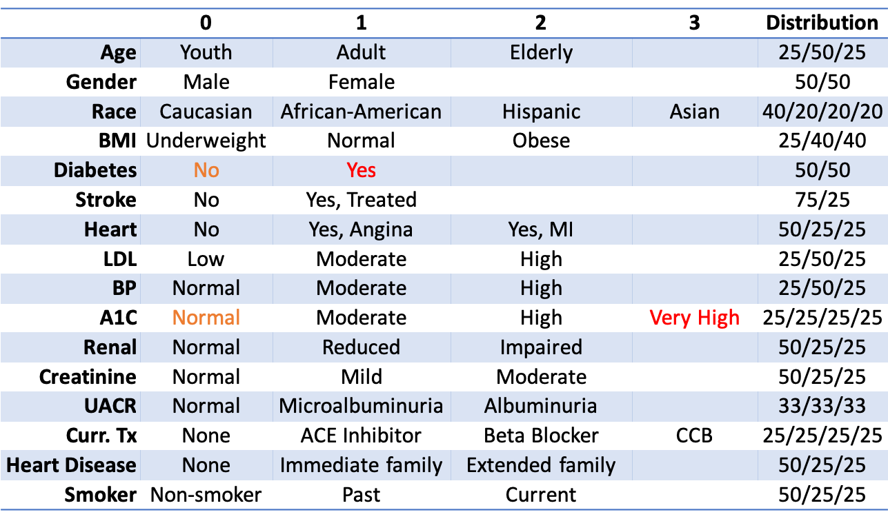
Among the attributes are a Type 2 Diabetes diagnosis (yes or no) and a given patient’s A1C levels (normal, moderate, high, or very high). As T2D diagnosis and A1C are linked, we have the following interaction constraints: (1) Patients with normal A1C cannot have T2D, and (2) Patients with very high A1C must have T2D.

The candidate set for this problem has 30,233,088 different combinations. As before, we seek to reduce time-in-survey by creating a fractional-factorial design, this time consisting of 50 unique patient profiles. The 50-profile fractional-factorial design must be as efficient as possible.

Model Definition

where $N$ is the number of observations, $\delta$ are vectors of relaxation variables, and $X$ is the design matrix consisting of $A ^ { j }$ attributes:

$\left[ \begin{array} { c c c } { A _ { 1 } ^ { 1 } } & { \dots } & { A _ { 1 } ^ { 16 } } \\ { \vdots } & { \ddots } & { \vdots } \\ { A _ { N } ^ { 1 } } & { \dots } & { A _ { N } ^ { 16 } } \end{array} \right]$

With decision variables $A ^ { 1 \ldots 16 }$ representing attributes:

$\qquad$ Age: $A _ { i } ^ { 1 }, \quad A \in \{ 0,1,2 \} , i = 1 , \ldots , n$
$\qquad$ Gender: $A _ { i } ^ { 2 }, \quad A \in \{ 0,1 \} , i = 1 , \ldots , n$
$\qquad$ Race: $A _ { i } ^ { 3 }, \quad A \in \{ 0,1,2,3 \} , i = 1 , \ldots , n$
$\qquad$ BMI: $A _ { i } ^ { 4 }, \quad A \in \{ 0,1,2 \} , i = 1 , \ldots , n$
$\qquad$ T2D: $A _ { i } ^ { 5 }, \quad A \in \{ 0,1 \} , i = 1 , \ldots , n$
$\qquad$ Stroke: $A _ { i } ^ { 6 }, \quad A \in \{ 0,1 \} , i = 1 , \ldots , n$
$\qquad$ Heart: $A _ { i } ^ { 7 }, \quad A \in \{ 0,1,2 \} , i = 1 , \ldots , n$
$\qquad$ LDL: $A _ { i } ^ { 8 }, \quad A \in \{ 0,1,2 \} , i = 1 , \ldots , n$
$\qquad$ BP: $A _ { i } ^ { 9 }, \quad A \in \{ 0,1,2 \} , i = 1 , \ldots , n$
$\qquad$ A1C: $A _ { i } ^ { 10 }, \quad A \in \{ 0,1,2,3 \} , i = 1 , \ldots , n$
$\qquad$ Renal: $A _ { i } ^ { 11 }, \quad A \in \{ 0,1,2 \} , i = 1 , \ldots , n$
$\qquad$ Creatine: $A _ { i } ^ { 12 }, \quad A \in \{ 0,1,2 \} , i = 1 , \ldots , n$
$\qquad$ UACR: $A _ { i } ^ { 13 }, \quad A \in \{ 0,1,2 \} , i = 1 , \ldots , n$
$\qquad$ Tx: $A _ { i } ^ { 14 }, \quad A \in \{ 0,1,2,3 \} , i = 1 , \ldots , n$
$\qquad$ Heart Hist: $A _ { i } ^ { 15 }, \quad A \in \{ 0,1,2 \} , i = 1 , \ldots , n$
$\qquad$ Smoker: $A _ { i } ^ { 16 }, \quad A \in \{ 0,1,2 \} , i = 1 , \ldots , n$

Again using the Dantzig-Wolfe reformulation to rewrite our integer variables, $Z$ represents the binary variable series replacing an integer variable, and $k$ represents the integer set of levels permissible for the given attribute:

$A _ { i } ^ { j } = \sum _ { 0 } ^ { k _ { j } } k Z _ { k } ^ { j } , \quad \text { and } \quad \sum _ { 0 } ^ { k _ { j } } Z _ { k } ^ { j } = 1 , \quad Z _ { k } ^ { j } \in \{ 0,1 \} , k ^ { j } \in A ^ { j }$

Subject to:

$\qquad$ Age group proportions (example) :

$\begin{aligned} \frac { \Sigma z _ { 0 } ^ { 1 } } { N } & = .25 + \delta _ { d } ^ { A 0 } \\ \frac { \sum Z _ { 1 } ^ { 1 } } { N } & = .5 + \delta _ { d } ^ { A 1 } \\ \frac { \sum Z _ { 2 } ^ { 1 } } { N } & = 25 + \delta _ { d } ^ { A 2 } \end{aligned}$

$\qquad$ … etc.

$\qquad$ Interaction constraints (T2D diagnosis and A1C level):

$\begin{array} { l } { Z _ { 0 } ^ { 5 } + Z _ { 3 } ^ { 10 } = 1 + \delta _ { i } ^ { 1 } } \\ { Z _ { 1 } ^ { 5 } + Z _ { 0 } ^ { 10 } = 1 + \delta _ { i } ^ { 2 } } \end{array}$

Conclusion

Results & Performance

The real-world problem is much too large for our implementation of the Fedorov Algorithm. With over 1 trillion swaps to calculate per iteration, the problem would take far too long to run to be useful. However, the larger problem space provides an opportunity to the improvement parallelization brings to our genetic algorithm. With lambda=1, the initial design has d-optimality 22.9. With lambda=0, the initial design has ¬d-optimality 59.9. Results are in the table below:

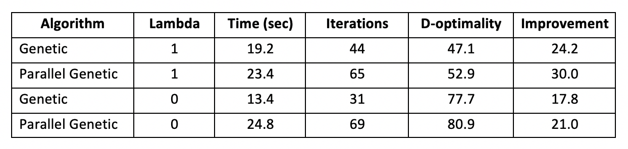
We see that the parallel genetic algorithm performed slower than the non-parallelized version but found improved designs. Additionally, these tests were run with population 100 and limited to 1000 generations. Tests with larger populations would likely begin to favor the parallel algorithm. Hypothetically, tests with more generations would also favor the parallel algorithm; however, we came nowhere near the 1000 generation limit in this test.

Takeaways & Next Steps

It is clear that for even moderately sized problems, the Fedorov Algorithm is unrealistic, regardless of whether we add additional constraints. We could address this by implementing some sort of preprocessing using the constraints to generate only feasible designs or reduce the candidate set only to feasible combinations before you begin the Fedorov iterations. While this preprocessing may be time consuming, it would reduce the memory requirements for storing the entire search space.

Aside from the size constraints inherent to the Fedorov Algorithm, our modified Fedorov Algorithm seems to move in the wrong direction depending on the initial (random) matrix design. Upon review, we find that our code chooses poor swaps when updates cause singular or near-singular matrices.

Additionally, the way we implemented slack penalties for feasibility can cause problems as the eigenvalues may improve but be rejected due to feasibility. The multiplicative update to d-optimality is fairly natural given that it comes from a geometric mean. However, once we include the penalty, we start to have additive terms in the objective function. A multiplicative update doesn’t really work when, for example, lambda = 10 and the penalty term is bigger than the d-optimality term in the objective function. Our objective function starts negative and becomes more negative with each update because we favor positive deltas.

In both cases, we could implement a multistep update by checking unconstrained d-optimality, checking for a near/singular matrix result, and then applying the penalty term before deciding whether to swap or not. This would ensure that we only allow swaps that move our objective function in the correct direction, while choosing among that subset for swaps that are most feasible.

Bibliography

Hauser, J., & Rao, V. (2002, September). Conjoint Analysis, Related Modeling, and Applications. In IN MARKET RESEARCH AND MODELING: PROGRESS AND PROSPECTS: A TRIBUTE. Kluwer Academic Publishers.
Kuhfeld, W., Huber, J., & Zwerina, K. (1996, September). A General Method for Constructing Efficient Choice Designs. Retrieved October 2018, from https://faculty.fuqua.duke.edu/~jch8/bio/Papers/Zwerina%20Kuhfeld%20Huber.pdf
Labadi, L. A. (2015, February). Some Refinements on Fedorov’s Algorithms for Constructing D-optimal Designs. Brazilian Journal of Probability and Statistics, 29, 53-70.
Triefenback, F. (2008). Design of Experiments: The D-Optimal Approach and Its Implementation As a Computer Algorithm. Umeå University, Department of Computing Science.
Warren F. Kuhfeld. (2001, January). Multinomial Logit, Discrete Choice Modeling. Retrieved October 2018, from https://www.stat.auckland.ac.nz/~balemi/Choice.pdf