Capstone Project (MS Business Analytics)
Behavioral segmentation and forecasting based on natural gas consumption
Vineeta Agarwal, Pragati Awasthi, Alex Graber, Grace Li, Faiz Nassur, Khushbu Pandit, An Tran, Yi Zhu
Business Problem
A local utility company uses Rate Codes to help define the rates that accountholders pay for natural gas and electricity. Rate codes help the company correctly bill customers; rate codes are determined at the time of sign-up using best available data regarding expected use (commercial vs. residential, gas vs. electric heating, pool vs no pool). It is possible that a customer may not know all of their appliances or energy use needs when creating an account, leading to potential rate code misclassification. Additionally, customers within each rate code group may not have similar use patterns, leading to decreased accuracy when forecasting by rate code.
Billing is done based on use where use is defined at the local meter; electricity is billed based on kilowatt-hour (kWh) used, and gas is billed based on 100 cubic feet (CCF) used.
Data was provided by the local utility company. All PII was removed/obfuscated.
The objective of the project is to build and validate a customer segmentation based on the influence of weather to enable the company to create more accurate forecasts for natural gas consumption. The project scope includes:
- Understand current Rate Code segmentation and forecast applications
- Create a new segmentation based on the influence weather attributes have on natural gas consumption
- Identify the best forecast models for each segment
- Identify potential rate code mislabeling
Summary
Summary
- Retroactively adding account attributes such as magnitude of average use and response to temperature may support improved forecasting and billing abilities.
- Response to temperature must be defined over a timeframe that experiences temperate and cold temperatures (Sept – Feb).
- Segmenting by magnitude of average use reduces regression errors, but also requires a history of use over a timeframe that experiences both warm and cold temperatures.
- The few accounts in the ‘huge’ magnitude category have highly varied use, making forecasting as a cluster challenging.
- 83% of meters demonstrate temperature-driven gas consumption; these meters account for only 54% of total gas sold in 2018.
- The majority of meters are temperature-driven based on our analysis.
- Weather-based forecasting works well for these accounts, covering residential and small/medium commercial meters.
- A few (11) large, commercial accounts are not weather-driven and account for nearly half of the gas consumption Jan-Sept, 2018.
- Forecasting for these large accounts is challenging; use is not easily predicted by weather or history.
- The majority of meters are temperature-driven based on our analysis.
- Forecast models using prior temperature and change in temperature are sufficient to predict gas use for temperature responders.
- Among responder groups, the prior day’s lowest temperature and the change from day to day explains approximately 80% of the change in daily use.
- Hourly forecasts based on the prior hour’s low and change in temperature over the past 6 hours do not perform as well as a daily model.
- Weather-based forecasts require anticipated future temperatures to predict future use; we recommend using them in the near-term (potentially to improve spot-market purchase predictions).
- Models based on historic use do not perform any better than weather models, even on clusters that do not respond to weather.
- Weather models demonstrate significantly better performance on responder clusters, as opposed to non-responders or Rate Codes.
- When comparing clusters to Rate Codes, we identified a small proportion of customers who may be misclassified and need further investigation.
- 17% of residential meters and 3% of commercial meters exhibit average use < 1.5 CCF / day and are not responsive to weather. However, they are billed using the gas heat Rate Code.
- Of the accounts that have both a gas and electric meter, 14% are minimal gas users and not responsive to weather. However, they are billed using the electric non-heat Rate Code.
- Adding response to weather to the company’s current rate codes may help improve forecasting for responsive groups, and help identify potentially misclassified accounts.
Analysis and Modeling
Procedure
Procedure
Broadly speaking, our procedure for analysis and modelling consisted of 4 main steps (see Figure 1 below):
- Identify differing use patterns and group meter IDs according to similarity of use.
- Create forecasting models and identify optimal model for each cluster.
- Compare forecast accuracy from forecasts based on clusters to accuracy from forecasts based on rate code
- Identify accounts where actual patterns of use do not align with anticipated patterns inferred from rate codes.
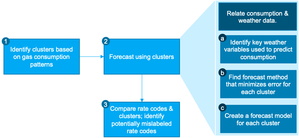
Figure 1. General procedural flow for analysis and modeling
Segmentation
Segmentation
Segmentation seeks to identify groups with similar behavior. As our task was to identify a weather-based model, we wanted to understand how each customer (meter ID) behaved with respect to weather. With that in mind, we created groups by answering the following questions: “On average, how much gas use does the meter read,” and “How does the metered use respond to changes in temperature?”
To understand how much gas each meter used, we calculated each meter’s average use from 2017 to 2018. Looking at the distribution of consumption, we defined 4 thresholds, creating 5 clusters where the meters in each group all have similar average daily use (see Figures 2,3):
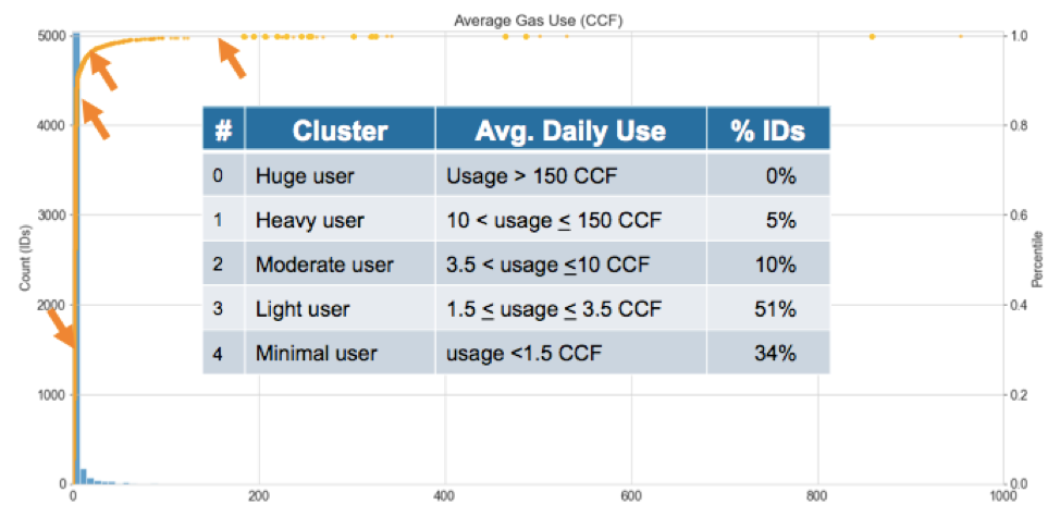 Figure 2. Five sections are defined based on Magnitude of average daily gas consumption
We expect residential and small commercial accounts to have relatively small daily usage, and only large commercial and industrial accounts to have high use. As 88% of our population are residential customers, it makes sense that we have a large population of customers who fall into minimal and low usage clusters.
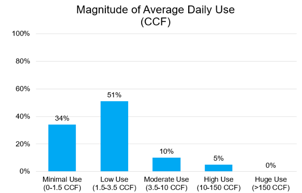 Figure 3. % of Population of Five clusters defined based on Magnitude of average daily gas consumption
In order to understand how use responds to weather, we had a hypothesis that as temperatures decrease, gas use should increase when it is used as a source of heating. Therefore, we looked at use from September 2017 to February 2018 as these months should exhibit temperature variation and also contain the coldest temperatures of the year. We then examined temperature vs average gas use for each date and meter. This allowed us to identify whether and how each meter’s use changes in response to the temperature.
The goal of clustering is to identify groups of meters that have similar behavior which we interpreted as similar weather responses. We used an algorithm called k-shape that identifies similarities between time-series data, allowing us to identify groups with similar behavior. Using k-shape, we identified 2 clusters (see Figures 4, 5) based on whether their gas consumption is responsive to temperate and cold temperatures or not. The weather-responsive cluster demonstrates gas consumption with a directly inverse relationship to temperature. Clusters that do not directly respond to weather (‘non-responders’) may ignore large temperature swings, demonstrate high use that is not related to weather, or behave non-intuitively.
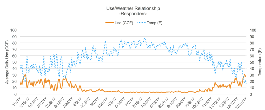
Figure 4. Weather responsive cluster
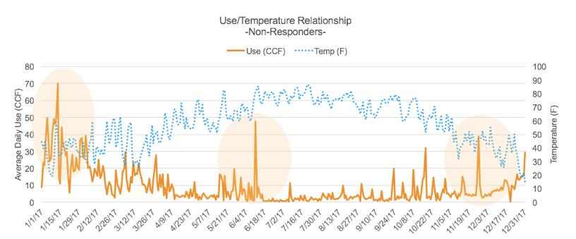
Figure 5. Non-responsive cluster
The majority (84%) of the meters in our data are responders (see Figure 6). As with the magnitude of use analysis, this makes sense as most of our meters belong to residential accounts, which primarily use natural gas for heating. When gas is used for heating, we would expect to see use increase as temperatures decrease.
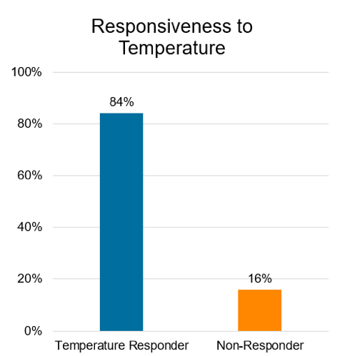
Figure 6. Percentage of Population of two clusters defined by responsiveness to temperature
Combining magnitude of use and response to temperature analyses, we identified 10 clusters (5 use, 2 response). However, no accounts exist in the low use non-responder category, leaving us with 9 clusters, of which the largest cluster has low average use (1.5-3.5 CCF per day) and responds to weather.
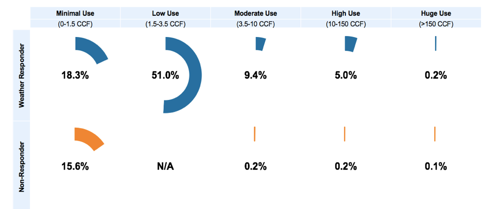
Figure 7. 9 clusters based on magnitude of use and response to temperature
Understanding New Clusters
Understanding New Clusters
Within residential customers, 17% are non-responders with minimal usage (see circle in Figure 8 below), and all have a heating rate code, which indicates potential of misclassification and would require further investigation.
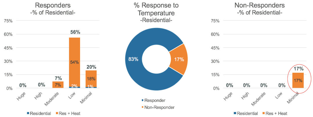
Figure 8. Residential customers
Most commercial accounts are responsive to weather; the exceptions are primarily commercial ‘transport’ accounts for whom PECO merely provides transportation for natural gas. The accounts generally have huge consumption, and likely do not use natural gas for heating, perhaps instead using for industrial purposes.
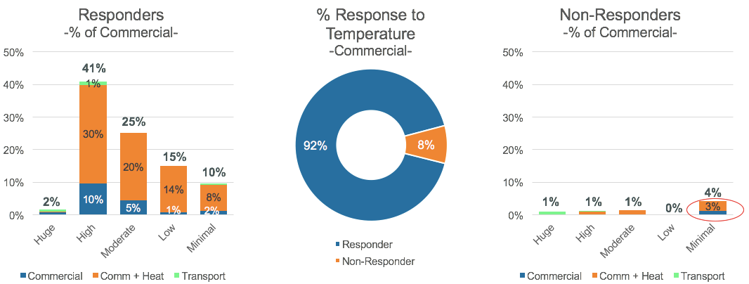
Figure 9. Commercial customers
For accounts with both a gas and an electric meter, we identified some potential misclassification as 14% of the accounts that have both a gas and electric meter use minimal amounts of gas and do not respond to weather are billed using the electric non-heat rate code. We believe these accounts do not use gas for heating; they may use oil, wood, or electricity instead. If these accounts use electric heating, they are misclassified.
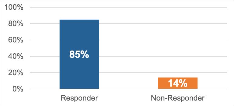
Figure 10. Comparing new cluster with Electric Rate Code (all displayed are non-heat rate codes)
The dual-service accounts (one with both electric and gas meters) with minimal non-responsive gas usage, 3% have both gas and electric heat rates or neither.
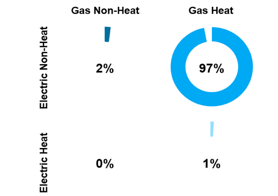
Figure 11. Merging gas with electric heat rate code for residential accounts
Forecasting
Forecasting
We implemented both regression models and time-series forecasts on daily and hourly data. We investigated using any and all weather information as predictors of gas use in the regression model; however, only prior temperature and change in temperature demonstrated significant relationships with use. Plotting the relationship between use and temperature indicated a linear relationship, so the regression model is a linear regression predicting use based on prior temperature and temperature change (Figure 12). The daily regression model uses the prior day’s low temperature and the change from the prior day, while the hourly regression model uses the prior hour’s temperature and the change in temperature from 6 hours ago.
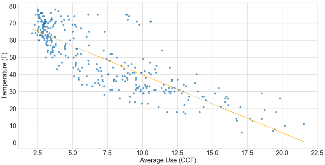
Figure 12. Relationship between temperature (F) and average use (CCF)
The time-series models were developed using an automated SARIMAX (Seasonal, AutoRegressive Integrated Moving Average with eXternal regressor) function that automatically identified the appropriate parameters for the models. The SARIMAX models use historic use, seasonal trends, and temperature as predictive inputs to forecast use.
At the daily level the regression models demonstrate good explanation among Responder groups, with an R2 value of approximately 80% across all responder groups. However, the regression models have low R2 values and high error (RMSE: Root Mean Square Error – lower is better) for non-responder groups (Figure 13). We attempted to use the SARIMAX models as an alternative forecast method for clusters where regression forecasts do not perform well. Unfortunately, SARIMAX models did not perform any better on these groups, which can be due to (a) insufficient historic data to detect trends/patterns, or (b) that these clusters’ natural gas use is triggered by an external factor that is not presented in the dataset.
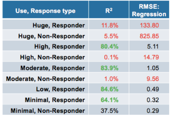
Figure 13. Error metrics for daily forecast models
We created similar Regression and SARIMAX models for hourly data, which did not perform as well as on daily level. This is to be expected, as there is more variability (and thus, unpredictability) as the granularity of the data increases. We see the same problem with hourly as we did with daily data - among Responder groups, approximately 60% of the change in use can be predicted using the prior hour’s low (°F) and the temperature change over the past 6 hours. However, the models still do not perform well on clusters that have “huge” usage and other clusters who do not respond to temperature.
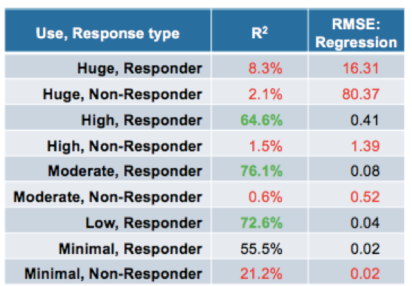 Figure 14. Error metrics for hourly forecast models
In both daily and hourly forecasts, “huge” users are very challenging to forecast. Part of this problem is that the average use per meter varies between 150 CCF to >4000 CCF. This dramatic variance within the “huge” group means contributes to the high error rate. Additionally, the small number of “huge” meters mean that each meter can have a large influence on the average. It may be that forecasting each meter individually gives better results, especially for the “huge” meters with a weather response.
Based on our analysis, we believe that retroactively adding attributes about magnitude of average use and response to temperature to customer accounts may support improved forecasting and billing abilities. Response to temperature must be defined over a timeframe that experiences temperate and cold temperatures (September-February). Segmenting by magnitude of average use reduces regression errors but also requires a history of use over a timeframe that experiences both warm and cold temperature.
Conclusion
83% of the meters in our sample have use that responds to weather, meaning they are viable candidates for weather-based regression forecasts. These accounts consist primarily of residential and small commercial meters. However, this 83% of meters accounts for only 54% of total gas sold in 2018 (Figure 15). The relatively few commercial accounts that are non-responsive to weather but have huge/high use account for nearly half of the gas consumption January- September 2018, and these commercial accounts have highly varied usage, which makes forecasting as a cluster challenging as their use is not easily predicted by weather or historic consumption data.
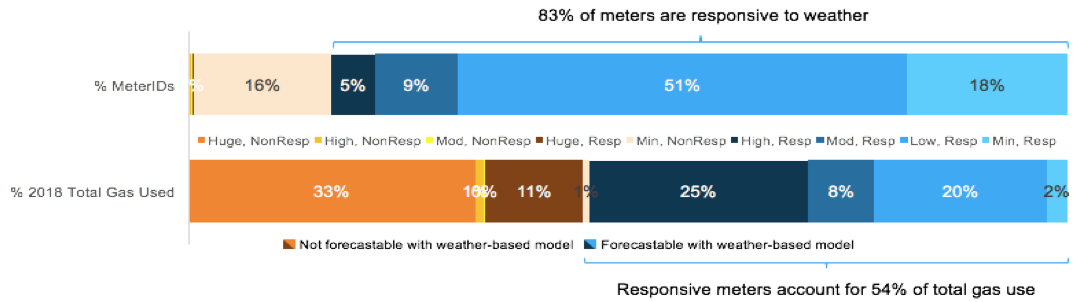
Figure 15. Meter responsiveness and consumption
Regression forecast models using prior temperature and change in temperature on daily level are sufficient to predict usage for weather responders. Among responder groups, the prior day’s lowest temperature and the change from day to day explains approximately 80% of the change in daily use. Hourly forecast based on the prior hour’s low and change in temperature over the past 6 hours have slightly worse performance than the daily model. Time-series models based on historic use do not perform any better than weather-based models, even on clusters that do not respond to weather.
When comparing clusters to Rate Codes, we identified a small portion of customers who may be misclassified and need further investigation. Specifically, 17% of Residential meters and 3% of Commercial meters exhibit average use <1.5 CCF/ day and are not responsive to weather. However, they are billed using the Gas Heat rate code. Of the accounts that have both a gas and electric meter, 14% are minimal gas users and not responsive to weather, but they are billed using the Electric Non-heat rate code. Therefore, adding response to weather to the company’s current rate codes may help improve forecasting for responsive groups, and help identify potentially misclassified accounts.
Caveats & Limitations
Caveats & Limitations
The clustering technique using magnitude of average daily usage and response to temperature both require at least 9 months of contiguous use data per meter. They are best thought as a validation for the rate code, not as a replacement.
The technique used to identify response to temperature requires analyst experimentation and interpretation as we currently do not have a way to use current clusters to sort new meters. This requires analyst intervention any time new meters are acquired.
Weather-based regression requires future weather data to predict use, which incorporates the error from weather forecast models. Our forecast models are weak to data that varies without cause/ explanation (ex: huge usage cluster). ARIMA models are inherently data-greedy, and acquiring additional historic data may improve ARIMA performance for non-responsive clusters.